
Cash-Settled Compute Futures: Mechanics of a Neocloud Short Hedge
American Innovation Exchange (AI Exchange) will soon launch, making its GPU compute futures available to U.S. investors, pending regulatory review. This post walks through a futures trade from the perspective of a neocloud hedging forward unsold capacity.
Background
Below is a single fully-worked numerical trading example from the perspective of a neocloud operator using a short futures position to lock in the forward sale price of capacity it expects to have available but has not yet contracted to end customers. The example illustrates position sizing, daily mark-to-market, variation margin, cash settlement under two states of the world, and the residual risks that remain after hedging.
The futures contract used in this example is cash-settled. At expiration, the position's P&L is marked to the settlement value derived from the reference index. Cash settlement is the standard convention for commodity derivatives whose underlying is a service or a non-storable, non-deliverable quantity, and compute time falls into this category.
Architect, the parent company of AI Exchange, will also offer ComputeConnect, an exchange-for-physical mechanism for converting positions into actual compute capacity. In a future post, we will detail how a cash-settled future can be converted to actual compute capacity using EFPs.
Contract Specification
The following specification is an example of how a single-accelerator, cash-settled compute future could be constructed. The actual contract unit, tick size, and margin parameters of any listed contract are set by the futures exchange and its clearing house.
| Underlying | NVIDIA H100 rental-price index |
| Price quotation | U.S. dollars per GPU-hour |
| Contract unit | 10,000 GPU-hours |
| Minimum price fluctuation | $0.001 per GPU-hour = $10.00 per contract |
| Contract months | Monthly, extending along the forward curve |
| Settlement method | Cash settlement against the final settlement value of the reference index |
| Final settlement value | Published index level for the delivery period on the last trading day |
| Initial margin | $6,000 per contract |
| Maintenance margin | $4,800 per contract |
The Hedging Problem
A neocloud is, in commodity terms, a producer: it holds an inventory of accelerators and sells their output — compute time — to customers. Its economic exposure resembles that of any producer holding unsold inventory. If the market rental rate for H100 capacity declines before the operator has contracted its available GPU-hours, the revenue realized on that capacity falls. The operator is therefore long the physical commodity and bears the risk of a price decline.
The standard remedy is a short hedge: the producer sells futures in a quantity that approximates its unsold physical exposure. A decline in the market rate reduces physical revenue but produces an offsetting gain on the short futures, because a short position profits when the futures price falls. A rise in the market rate does the reverse. In both directions the combined outcome converges toward a price fixed at the outset, converting an uncertain forward revenue into a substantially known one. This is the mechanism by which a producer "locks in" a forward sale price without having yet found a counterparty for the physical product.
When executed properly, a compute futures hedge removes price variance from a defined block of capacity so that build-out, financing, and margin commitments can be underwritten against a known revenue figure.
Establishing the Position
Assume the following facts as of the trade date:
- The operator projects 500,000 H100 GPU-hours of uncontracted, saleable capacity during the March 2027 delivery window.
- The March 2027 H100 future is trading at F₀ = $2.40 per GPU-hour.
- The operator wishes to fix the revenue on the full 500,000 GPU-hours at the prevailing forward level.
Number of contracts. The hedge quantity is the physical exposure divided by the contract unit:
N = 500,000 GPU-hours ÷ 10,000 GPU-hours/contract = 50 contracts
The operator sells (goes short) 50 March 2027 H100 futures at $2.40 per GPU-hour.
Notional value hedged:
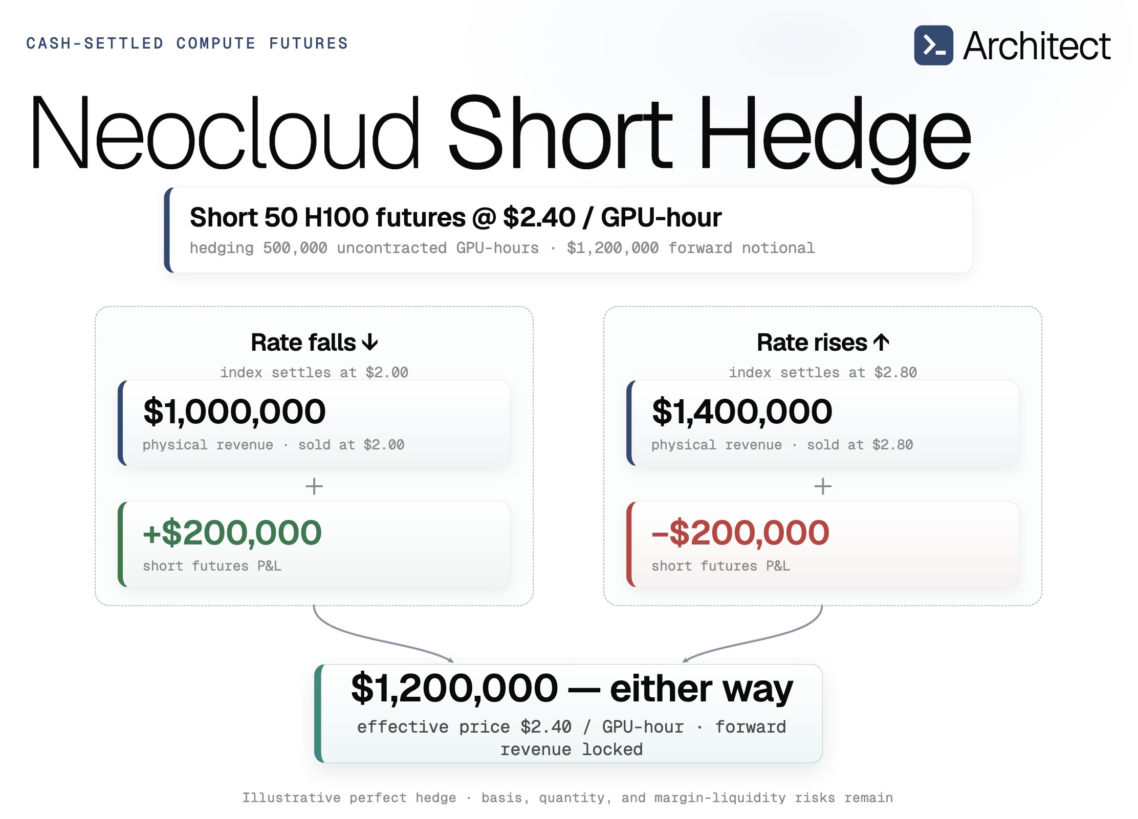
50 × 10,000 × $2.40 = $1,200,000
Initial margin posted:
50 × $6,000 = $300,000
The $300,000 is a good-faith performance bond held with the clearing broker (FCM), not a payment for the contracts. It is returned when the position is closed, adjusted for accumulated gains and losses. The economic significance of the position is the $1,200,000 of forward revenue whose price has now been fixed, posted against 25% of that sum in initial margin — illustrating the capital efficiency of a marginable hedge relative to pre-selling the capacity outright.
Daily Mark-to-Market and Variation Margin
Futures positions are marked to market at the close of each trading session. The change in the settlement price is converted into a cash flow called variation margin that is debited from or credited to the position holder's account daily. For a short position, a fall in the futures price produces a credit and a rise produces a debit. The following two sessions illustrate the mechanism.
| Session | Settlement price | Variation margin | Account equity | Margin call? |
|---|---|---|---|---|
| Session 1 | $2.34 (−$0.06) | +$30,000 | $330,000 | No — excess available for withdrawal |
| Session 2 | $2.60 (+$0.26) | −$130,000 | $200,000 | Yes — equity below $240,000 maintenance; restore to $300,000 |
After Session 2, the FCM issues a margin call requiring the operator to restore equity to the initial margin level of $300,000 with a payment of at least $100,000. This intraperiod cash demand illustrates the financing consideration addressed in Section 7.
Cash Settlement at Expiration
On the last trading day the contract is settled in cash against the final settlement value of the reference index for the March 2027 window, denoted St. The cumulative profit or loss on the short futures position is:
Futures P&L = (F₀ − St) × 500,000
This figure is the algebraic sum of all daily variation-margin flows over the life of the position; the final session's mark simply brings the futures price into convergence with the settlement index. In parallel, the operator sells its 500,000 uncontracted GPU-hours into the physical market at the prevailing rate, taken here to equal the settlement index. Two scenarios are considered:
| Scenario A — Rate declines (St = $2.00) | Scenario B — Rate rises (St = $2.80) | |
|---|---|---|
| Physical revenue | 500,000 × $2.00 = $1,000,000 | 500,000 × $2.80 = $1,400,000 |
| Futures P&L | ($2.40 − $2.00) × 500,000 = +$200,000 | ($2.40 − $2.80) × 500,000 = −$200,000 |
| Combined proceeds | $1,200,000 | $1,200,000 |
| Effective realized price | $2.40 / GPU-hour | $2.40 / GPU-hour |
In both scenarios the effective realized price is $2.40 per GPU-hour — equal to the futures price at which the hedge was established. This symmetry is the defining characteristic of a fully executed short hedge: the operator has exchanged all upside above $2.40 for complete protection below it, fixing the forward revenue on the hedged block of capacity regardless of the direction of prices.
Hedge Effectiveness and Residual Risks
The example above assumes a perfect hedge, in which the price realized on the physical capacity equals the settlement index, and the hedged quantity equals the quantity ultimately sold. In practice, two residual exposures remain.
Basis risk
The rate the operator actually realizes on its own capacity, Rt, need not equal the settlement index level, St, because the index aggregates transactions across many configurations, geographies, and counterparties. The effective realized price generalizes to:
Effective price = Rt + (F₀ − St) = F₀ + (Rt − St)
where the term (Rt − St) is the basis. If, for instance, the operator realizes $1.95 per GPU-hour while the index settles at $2.00, the effective price becomes $2.40 + ($1.95 − $2.00) = $2.35 rather than the intended $2.40. Basis risk is the price of standardization: a single index cannot perfectly track the heterogeneous rate a specific operator obtains, and the residual is borne by the hedger. Selecting the reference SKU and delivery window that most closely matches typical physical exposure minimizes, but does not eliminate, this term.
Volumetric risk
The contract count is fixed at inception on the basis of a projection of saleable capacity. If the operator ultimately has only 450,000 saleable GPU-hours rather than 500,000, it is over-hedged by 50,000 GPU-hours — five contracts — and that slice of the short position is no longer offset by any physical inventory. It becomes an outright short exposure to the compute price and produces an unhedged gain or loss. Conservative sizing — hedging a quantity at or below the highly probable minimum of expected saleable capacity — limits this exposure.
Liquidity and margin risk
As shown in the mark-to-market section above, an adverse move in the futures price requires variation margin to be posted in cash before the offsetting physical gain is realized. A hedge that is economically sound can still impose a financing burden during its life, and this must be provisioned for.
Summary
A cash-settled compute future allows a neocloud to fix the forward sale price of capacity it expects to have available but has not yet contracted. By selling a number of futures equal to its uncontracted GPU-hours divided by the contract unit, the operator establishes a short position whose daily and terminal profit-and-loss offsets the change in the value of its physical inventory. In the worked example, 50 March 2027 H100 contracts sold at $2.40 per GPU-hour fix the proceeds on 500,000 GPU-hours at $1,200,000, whether the rental rate subsequently falls to $2.00 or rises to $2.80.
The instrument converts an uncertain forward revenue into a substantially known one, subject to basis risk, volumetric risk, and the intraperiod liquidity demands of the margin system. For an operator underwriting build-out and financing commitments against future capacity sales, that conversion of variable revenue into a hedged forward curve is the central economic function of the trade.
New to compute futures? Start with Compute Futures, or explore how futures and perpetuals differ in Perpetuals vs Futures.
Trade compute futures on AI Exchange
AI Exchange is the first CFTC-regulated venue for futures on compute costs and other AI supply-chain inputs — currently pending regulatory review.
Learn about AI ExchangeAmerican Innovation Exchange LLC ("AI Exchange") is registered with the Commodity Futures Trading Commission as a designated contract market, but is pre-operational. AI Exchange's intended products described herein will only be offered in compliance with all applicable law and regulations. This material is for informational purposes only and does not constitute an offer to buy or sell any financial instrument or a solicitation of any investment. Information is provided "as is" and any descriptions of planned products, features, or services are preliminary, subject to change without notice, and should not be relied upon as commitments regarding future availability, functionality, or performance. Trading futures involves substantial risk of loss and may not be suitable for all participants and may result in losses exceeding your initial investment amount. Leverage can amplify both gains and losses. Past performance is not indicative of future results. This material does not constitute investment, legal, tax, or regulatory advice. Recipients should conduct their own due diligence and consult qualified advisors before transacting. Not available where prohibited by law.